What is anomaly detection?
Anomaly detection is the process of identifying patterns in data that do not follow expected behaviour. These atypical patterns are called anomalies or outliers.
- Anomalies: Also known as outliers or unusual examples. These are the unexpected events in data.
- Normal examples: These are the typical, expected data points - also known as inliers.
Outliers themselves can fall under different categories:
- Outliers: Brief and irregular patterns in the data.
- Change in Events: Systematic or abrupt changes from the previous normal patterns.
- Drifts: Gradual, long-lasting shifts in the data.

Image created with DALL·E 3
Real-world applications of anomaly detection
From finance to healthcare, anomaly detection is applied in countless real life use cases and can be used in both contexts of preventive analysis and predictive analysis. Here are just a few examples:
- Fraud detection: Identifying suspicious patterns in customer credit card transactions for fraud before accounts are emptied
- Finance: Spotting unusual trading patterns in stock markets
- Manufacturing quality assurance: Catching defects parts using IoT sensor data and computer vision to prevent costly recalls
- Machine learning: Outliers can affect the performance of forecasting models
- Industrial equipment monitoring: Detect anomalies in telecom network tower systems to predict failures and reduce downtime
- Health monitoring wearables: Your smart watch can warn you on potential health issues based on your irregular heart rates
- E-commerce: Detecting hacked accounts through suspicious customer purchasing behaviour
- Streaming services: Companies such as Netflix and Spotify can detect account sharing or unauthorised actions
- Network security: Detecting unusual system behaviours may indicate a cyber-security breach
Types of anomaly detection methods
There are many types of anomaly detection methods, which will be discussed in upcoming posts:
- Statistical Methods:
- Parametric Methods: These traditional methods, such as Z-score, assume that the normal data follows a certain distribution, typically Gaussian. Anomalies are then identified as observations that are unlikely under this distribution.
- Non-Parametric Methods: Do not make any assumptions about the underlying distribution of the data. Examples include Tukey’s Fences and the Median Absolute Deviation (MAD).For Tukey’s Fences, any points that lie outside 1.5 times the IQR (Interquartile Range) (above the third quartile or below the first quartile) are deemed anomalous.
- Supervised Learning Methods
- Classification Models treat anomaly detection as a binary classification problem. Models like Logistic Regression, Decision Trees, or Neural Networks are trained on labeled data to distinguish between normal and anomalous instances.
- Regression Models, such as Linear Regression and XGBoost (eXtreme Gradient Boosting), predict a numerical value for each data point and consider points with high prediction errors as anomalies.
- Semi-Supervised Learning Methods:
- Neural networks, like autoencoders, can be used to reconstruct normal data. When these methods encounter an anomaly, the reconstruction error is high, signalling an anomalous data point.
- One-Class SVM uses Support Vector Machines to find the hyperplane that best separates the data from the origin. Data points far from the hyperplane are considered anomalies.
- GMM (Gaussian Mixture Model) fits multiple Gaussian distributions to the data. Points that fall into low-probability Gaussians can be considered anomalies.
- Unsupervised Learning Methods:
- Density-Based Methods:
- DBSCAN (Density-Based Spatial Clustering of Applications with Noise) compares the density around a data point with the density around its neighbours. Anomalies are located in regions with significantly lower density.
- LOF (Local Outlier Factor) measures the local deviation of a density of a data point with respect to its neighbours. Higher LOF value indicates an anomaly.
- Distance-Based Methods:
- These methods, like KNN (k-Nearest Neighbours), assume that normal data points occur in dense regions, while anomalies are far from their nearest neighbours. In KNN, each data point has its distance to its kth-nearest neighbor computed. If the distance is above a certain threshold, the point is considered an anomaly.
- Ensemble Methods:
- Tree based models such as Isolation Forest build multiple decision trees by randomly selecting features and splitting values, isolating anomalies more quickly than normal points.
- Density-Based Methods:
- Time-Series Methods:
- Statistical Process Control (SPC) uses control charts to monitor the stability of a time-series and detect anomalies.
- ARIMA-Based Methods fit an ARIMA (Autoregressive Integrated Moving Average) model to the time-series data and identify anomalies as points that have high residuals.
- LSTM Neural Networks use Long Short-Term Memory networks to model complex temporal dependencies and identify anomalies based on prediction errors.
- Random Cut Forest models work similarly to Isolation Forest but are designed to work with streaming data.
- Hybrid Methods:
- These methods, such as Feature Bagging, combine multiple anomaly detection algorithms, often leveraging their individual strengths to improve overall performance.
Statistical methods are a useful heuristic starting point for anomaly detection. However, in real life scenarios where the downstream consequences of a false positive or false negative has serious consequences to a company’s bottom line or someone’s health, then more sophisticated techniques are required.
How does anomaly detection work?
Anomaly detection algorithms are unsupervised machine learning algorithms that look at an unlabelled dataset of normal events and learn to detect unusual or anomalous events by modelling. The anomaly detection algorithm tries to find brand new positive examples that may be unlike anything previously seen.
A popular anomaly detection technique is density estimation, as it is flexible and intuitive. To illustrate, let’s use an example in the manufacturing domain where we are detecting faults in the Electric Vehicle (EV) battery manufacturing. Here a positive case ($y=1$) is when a battery fault is detected, and a negative case ($y=0$) is when a battery is normal / good without faults.
Typically we will have some labelled data of normal and anomalous examples. Let’s say we have a dataset with 5k normal batteries and 10 faulty batteries. We could split this dataset into three parts:
- Training set - 3k normal examples
- Cross-validation set - 1k normal examples, 5 anomalies
- Test set - 1k normal examples, 5 anomalies
Let’s say that within the dataset, there are two features used to predict battery faults:
- $x_1$ = battery temperature (°C)
- $x_2$ = battery voltage (Volts)
This is considered an unsupervised or semi-supervised learning algorithm because the training sets have no labels or are labelled as normal ($y=0$).
Alternative method: No test set, i.e. only use a training set and cross-validation set
This option is usually only considered when you have very few anomalous examples, such as 2 positive classes. The main downside of this option is that you do not have a fair way of assessing how well the algorithm will do in future examples. Also, there is a greater chance of the algorithm overfitting, thus performance on real data may be lower than expected.

Image created with Leonardo.AI
Gaussian distribution: A quick recap
The Gaussian distribution, or Normal distribution or bell curve distribution, is a curve that describes how data clusters around a central value, with fewer values appearing as you deviate away from this central value in either direction. Gaussian distributions have two parameters:
- $μ$ (Mu): This is the mean of the data and the central point of the curve
- $σ^2$ (Sigma squared): This is the variance - a measure of how spread out the data is. If the variance is small then the data is closely packed around the mean. If the variance is large, then the data is more spread out. This is because the area under the curve, probability density function (PDF), always equals 1. The standard deviation ($σ$) is used to describe the width of the bell curve.
In anomaly detection, we often assume our “normal” data follows a Gaussian distribution, meaning that most “normal” data points will cluster around the mean and the further we move from the mean, the fewer data points there are.
Using density estimation, we can calculate the probability of a new data being “normal” by estimating the PDF of a random variable based on observed data. If this new data point lies far from the mean and beyond a certain threshold, its probability under the Gaussian distribution will be very low, and may be considered an anomaly.
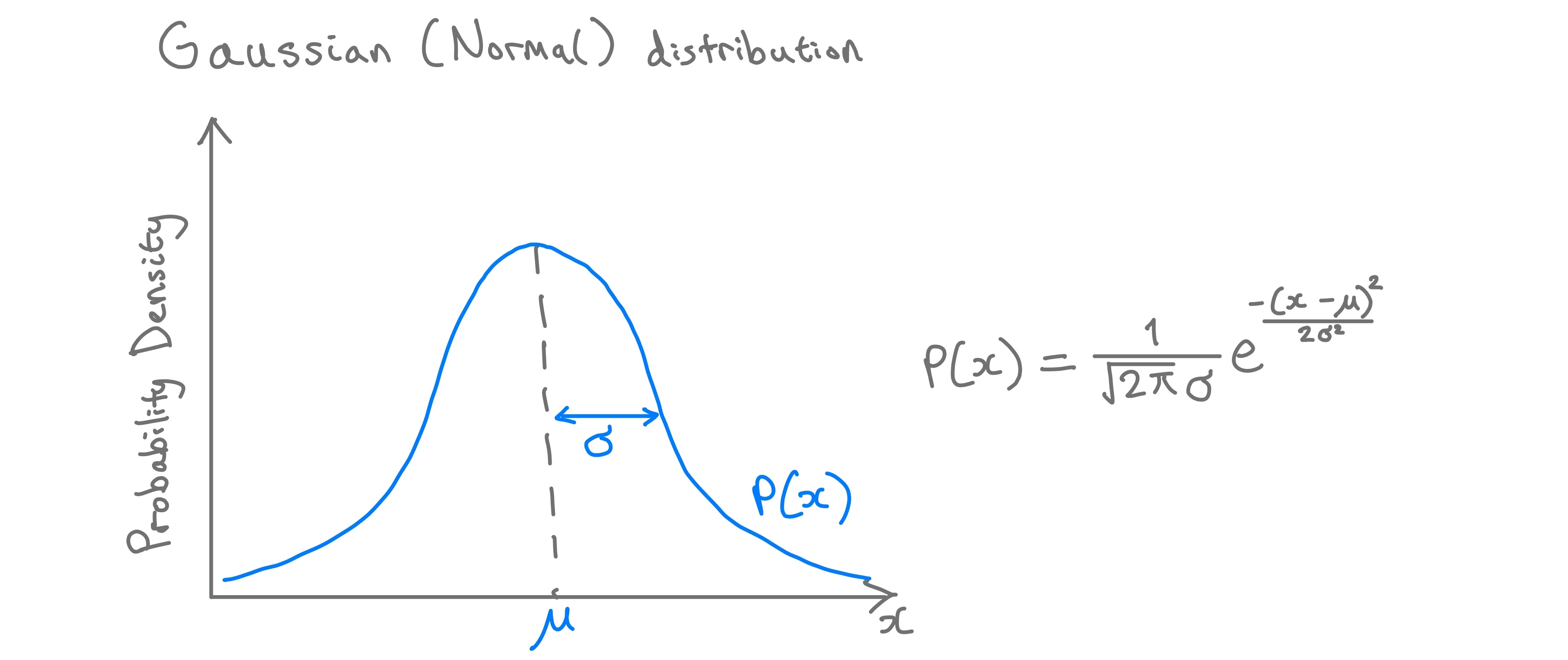
Gaussain distribution and formula. Image by author.
Developing and evaluating an anomaly detection algorithm
Here is an overview of the steps in developing an anomaly detection algorithm for our EV battery example:
- Model the normal data: The algorithm is trained on the unlabelled training set,
- Where a Gaussian distribution is fitted on the 3k examples {$x^{(1)}, x^{(2)}, …, x^{(3000)}$ to model the probability of $x$, given by $P(x)$.
- Intuition: Here the model is learning what values of $x_1$ and $x_2$ have high and low probabilities of occurring.
- The model will fit parameters $μ_1, …, μ_n, σ_1^2, …, σ_n^2$.
- Compute the Density for the New Data: Give this trained model the unseen cross-validation data (1k normal and 5 anomalies) and compute the probabilities of $x_{test}$, $P(x_{test})$.
- Thresholding: Set a threshold parameter, $ε$ (epsilon), to predict $y=1$, whereby if $P(x$test $) < ε$ then the data point is considered an anomaly. This cross-validation set is used to tune and adjust $ε$ to detect the 5 anomalies, whilst minimising the flagging of normal batteries as faulty anomalies - false positives.
- Evaluate performance: Now we assess if the cross-validation and test predictions match the true $y$ labels. Take the algorithm and evaluate on the test set to see how many of the remaining 5 anomalous batteries it finds, and the number of false positive mistakes flagged by the algorithm.
- It is useful to create a confusion matrix consisting of the true positives, false positives, false negatives, and true negatives - to better understand the model performance
- For highly skewed data distributions, accuracy is a poor metric to evaluate model performance. Instead, common evaluation metrics for skewed data include precision, recall, and F1 score.
This is a systematic way of quantifying whether or not a new example $x_{test}$ has any features $x_1, …, x_n$, that are unusually large or small.
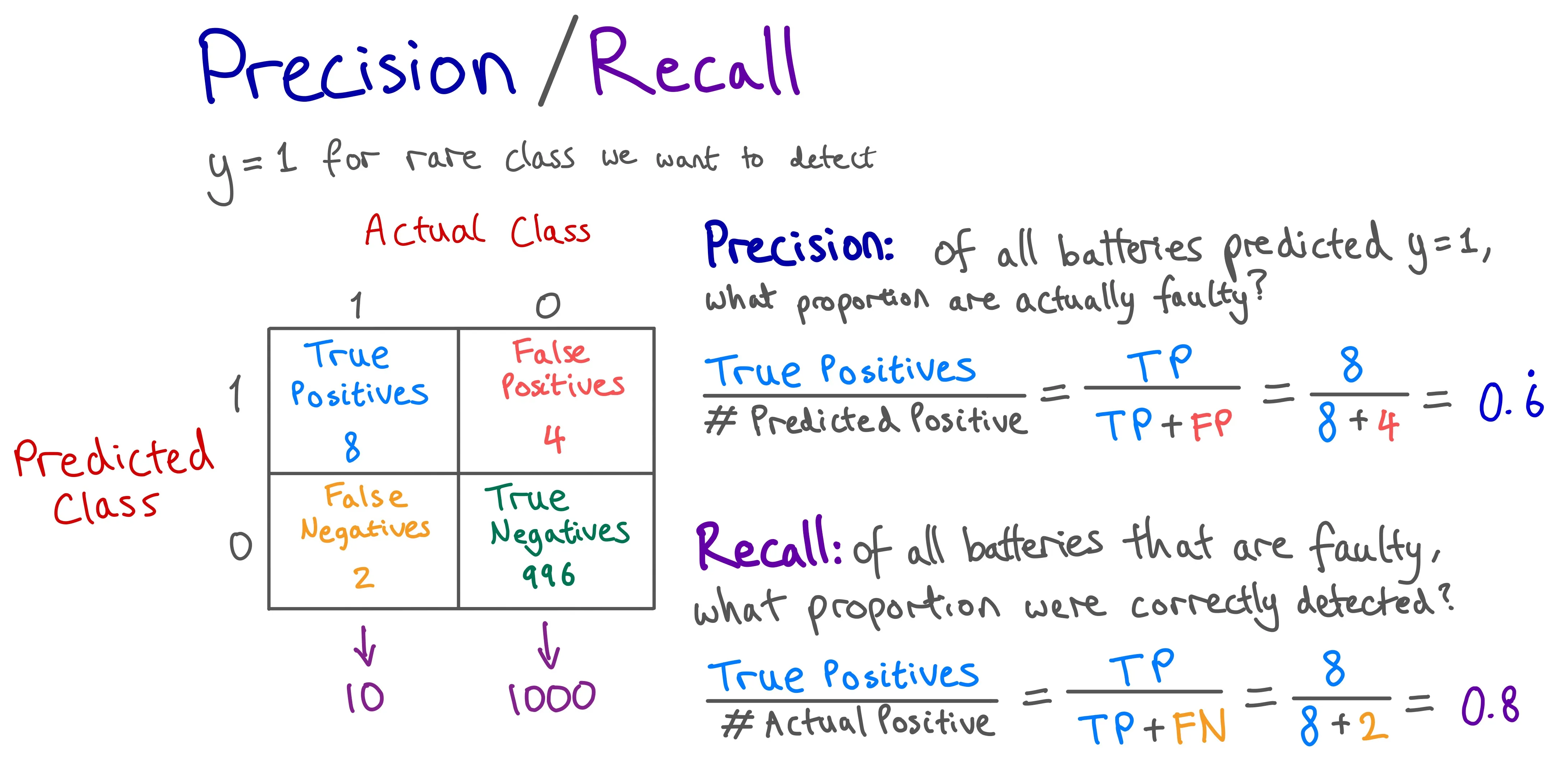
Example of calculating the precision and recall from a confusion matrix. Image by author
Improving model performance with feature selection
Two practical ways to improve model performance:
- Transforming non-gaussian features: Adjusting the data can help the model perform better.
- First, plot the distribution of a feature by plotting a histogram
- Apply transformations to $x_n$ to make it roughly fit a Gaussian distribution, such as applying $log(x_n+C)$ or applying a power.
- Note: Remember to apply these same transformations on the cross-validation and test sets as the training set.
- Error analysis: Identify where the model is going wrong and think of new predictive features that can help.
- With your domain knowledge, how do you know a certain example is anomalous. Can you think of a new feature that can distinguish a non-flagged anomalous example from the normal examples.
- The most common problem is that $P(x)$ is comparable for normal and anomalous examples, i.e. $P(x)$ is large for both. So, we need to choose features that take unusually large or small values in the event of an anomaly.
Anomaly detection vs Supervised Learning
The decision can be quite subtle when choosing an approach, as it depends on the specific application and nature of the data. For example, here are some considerations when deciding between anomaly detection and supervised learning algorithms.
| Category | Anomaly detection | Supervised learning |
|---|---|---|
| Intuition | The algorithm will flag an example as anomalous if one or more of the features are very large or very small relative to what it has seen in the training set. | The algorithm uses past positive examples to predict similar future positive examples. |
| When to use this approach | When the dataset has very few anomalous examples (0-20 positive instances is common) and many normal examples. Also used when there are many different “types” of anomalies, so that it is difficult for an algorithm to learn from past positive examples. | Used when there are a large number of positive and negative examples. So that there are sufficient positive examples for the algorithm to understand what positive examples are like, and future positive examples are similar to ones in the training set. |
| Example use cases | Security related themes are well suited, as bad actors are often trying to find new ways to hack into systems, like cybersecurity and financial fraud. Manufacturing: finding new previously unseen defects. There are many ways for an aircraft engine to go faulty, and a new type of fault may occur in future - the existing 20 examples do not cover new faults. | Email spam detection - although there are many types of spam email, they usually follow the same format of getting the recipient to click on a link or pushing them towards a certain action. Manufacturing: finding known previously seen defects Disease classification to predict if a patient has a specific disease |
| Feature engineering consideration | Anomaly detection learns from unlabelled data, so it is harder for the algorithm to learn which features to ignore. | Feature engineering for supervised learning is more forgiving, if features are not optimally tuned or if there are extra non-useful features then the model can still perform well. This is because the algorithm has the supervised signal that is enough to label Y for the algorithm to figure out which features to ignore, how to rescale features - to take advantage of the features provided. |
Conclusion
As you can see, anomaly detection impacts every facet of our lives and ensures the smooth running of many systems in our society. Hopefully this post has shown you:
- Why anomaly detection algorithms are useful across many domains
- How to develop an anomaly detection algorithm using density estimation
- What to consider when selecting an anomaly detection or supervised learning algorithm
Thanks for reading, I hope you’ve found this useful. Next time, I’ll be writing on the SOTA anomaly detection methods used in Kaggle competition winning notebooks, research papers, and leading AI blogs.
References
[1] Ng, Andrew, Bagul, A., Ladwig, G., & Shyu, E. Machine Learning Specialization: Advanced Learning Algorithms [MOOC]. Coursera. https://www.coursera.org/learn/advanced-learning-algorithms
[2] Ng, Andrew, Bagul, A., Ladwig, G., & Shyu, E. Machine Learning Specialization: Unsupervised Learning, Recommenders, Reinforcement Learning [MOOC]. Coursera. https://www.coursera.org/learn/unsupervised-learning-recommenders-reinforcement-learning
[3] Medico, Roberto. awesome-TS-anomaly-detection, (2023), GitHub repository, https://github.com/rob-med/awesome-TS-anomaly-detection
Acknowledgements
Thanks to Nirmalya Ghosh, Cecilia, Matthew, and Rosie for reading drafts of this post and providing feedback.